Tarantool data structures
This is the final part of a four-part transcript of my talk at Highload conference 2015. For the previous parts, see How tarantool works with memory, Tarantool engineering principles and Tarantool design principles.
I mentioned in Part 3 that Tarantool’s memory manager needs a feature usually called “consistent read views”: an instant snapshot of all allocated memory, which doesn’t change as the server goes along with creating and destroying objects.
To implement this feature, we created a data structure that is a mix of a B-tree container, an allocator and an address translation table. Having failed to find a single category for it, we, as it usually happens, aggravated the case by failing to choose a descriptive name, and called it matras. On a more serious note, it’s just a smart abbreviation for memory address translation. While we are at it, our allocators library is called small, which is short for small object allocation, our in-memory data structures are in a library called salad, which stands for specialized algorithms and data structures, our transaction log manager is called… well, you get the idea.
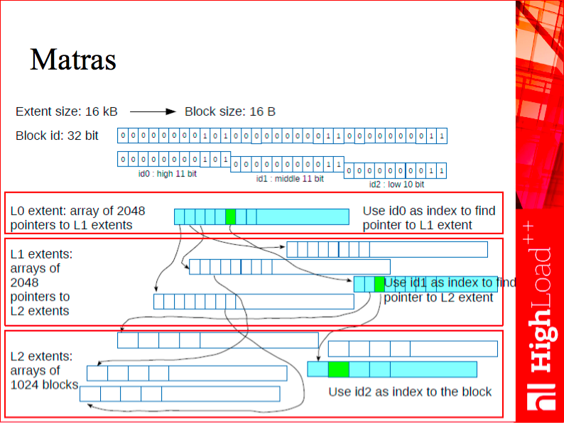
Matras is a kind of a user-space translation lookaside buffer (TLB), a system that allocates memory and translates addresses to the process address space, which is 32-bit in our case. Say, if we had a regular translator and needed to assign a 32-bit identifier to an 8-byte address, we would inevitably take up some extra memory for storing this mapping. We solve this problem by using the matras, which serves as both an allocator and a translation system. It allocates small objects that have to be of equal and aligned size; aligned size is a power of two (say, 16, 32 or 64 bytes), and returns its 32-bit identifier.
Internally, it is a three-level tree. The first level (let’s call it L0) has a root block that stores pointers to the second level (let’s call it L1) extents. The total number of these extents is 2048 since in the root block, we use the first 11 bits of a 32-bit number as extent identifiers. Once we get to an extent itself, that is to the second level of the tree, we can find where exactly our address is stored - that’s what the second 11 bits of the address are for. This allows us to go even deeper, and there already resides our allocated memory.
Due to restrictions on the object size, this data structure is not good for storing tuples or other general-purpose objects. But it is very good for such objects as B-tree pages or hash table buckets, and, as you know, in a database, every tuple eventually ends up either in a page of a tree or in a hash bucket.
Matras can maintain several consistent read views of its data. It’s a compact object (so compact that the L0 and L1 levels are almost certain to fit in the CPU cache), so we took a fairly straightforward approach to versioning it - the same technique as used in append-only B-trees. Now, to take a memory snapshot, we instruct this data structure to begin making copies of its L0, L1 and L2 objects each time there is an insert, update or delete request. Note, that these are only copies of the affected index pages, and as long as an in-memory database does not store data in the index, the data itself is not copied along. After we take a snapshot and release the consistent read view, we simply recycle the copies that have by now become garbage.
On the performance side, this data structure can execute about 10 million operations per second on average hardware configurations.
As I already mentioned, matras is at the core of all our indexes, to which I will now proceed.
A sneak peek into the future
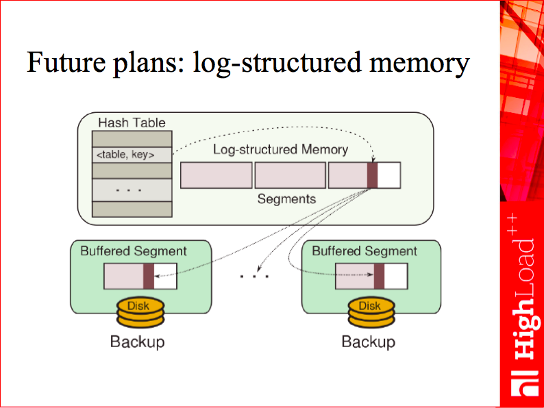
By the way, remember the log-structured allocator I mentioned earlier? We plan to begin using it for all our tuples in the future, by molding it with matras. If it’s possible to translate object addresses on the fly, why not just create a garbage collection-based allocator tailored to our needs?
This allocator might work as follows. To allocate a tuple, you simply look at free space in the most recently allocated chunk, and use it. You also remember the address of the object in matras, and return a matras id (32 bit) instead of a hardware address. Now, suppose you need to free a large chunk of memory, allocated long time ago. It’s mostly empty, but contains a few tuples that are still in use. With matras, you simply move the tuples to a fresh chunk, and update their addresses in a matras instance. Now you can free the old chunk. What’s great about this algorithm, is that it’s very easy to manage: you can reduce fragmentation by intensifying garbage collection, and you always know how much free memory is left. We’ve already built a prototype and plan to mature it in a future release.
Trees and hashes
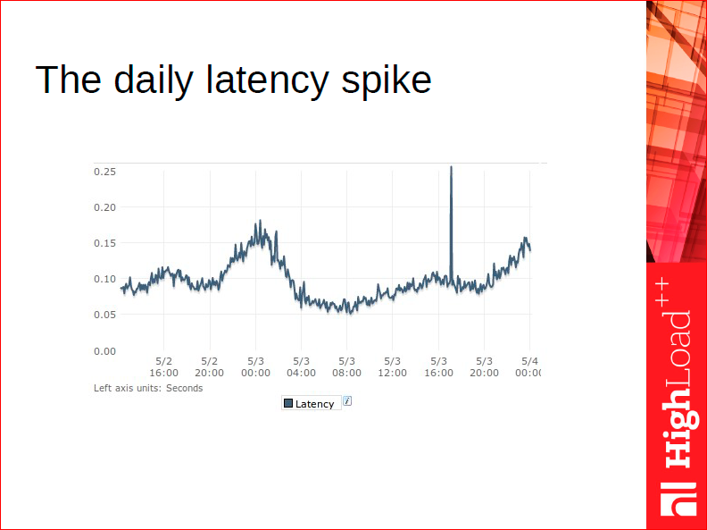
Before I start talking about our implementation of hashes, it’s worth telling a recurring story from my experience of working in an Internet company. An entry-level web developer knows very well that hashes are the fastest data structures with asymptotically constant lookup time. Cool, so they begin using hashes everywhere they can. They build another nifty little system, it goes live and then - the witch hunt begins. And by witches I mean these latency spikes that occur nobody knows when and why. People try to model the problem in a test environment and fail: the spikes only occur in production.
I’m being so sarcastic, because this situation is all too familiar. Picture a C++ developer who stores all the online users of a small (say, a few dozen millions) social network or a game in a hash. Then, say, in the evening, there’s an influx of new users to the site, which entails hash resizing. And while the hash is being resized, every user is waiting in the suspended mode - because our little nifty “online users hash” is used on every hit in the game - and that’s exactly the latency spike on the slide above. That’s the reason why using classical hashes for DBMSs is not a good idea: if you have a massive number of buckets, you just can’t afford hash resizing.
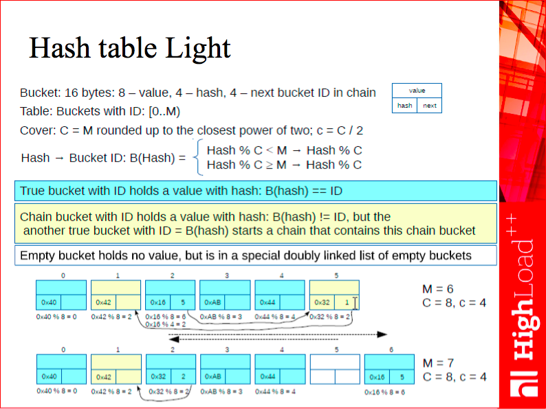
This is why our linearly expandable hash is never resized. To be more precise, it’s resized on each insert.
This data structure is based on a 16-byte bucket: 8 bytes are used for a pointer to a tuple, and two 32-bit numbers for the computed hash value and a pointer to the next element, respectively. You can see the structure in the upper right corner of the slide above.
The main parameter of our hash is a mask - it’s a power of two that fully covers the current hash size: if the hash contains 3 or 4 elements, the mask value is 4; for the hash of size 5, the mask value is 8. Thus, we have a virtual hash size that is resized in a regular manner. However, it’s just a number - in practice, we don’t materialize the bucket table, we simply add one element to our hash on each insert.
The second parameter of the hash table is a pointer to the current bucket that needs to be resized. Suppose our hash contains 2 elements, then the pointer to the current bucket is 0. We add a new element, split the 0th bucket and move the pointer to the next one. We then add another element, split the 1st bucket - as a result, we have 4 buckets, and we reset the mask and the resize counter. After that, we add a fifth element and split the 0th bucket - we now have 5 elements. In other words, we keep splitting from the beginning of the hash table until we reach the current value of the mask, then we double the mask and start over.
The difficult part of the story, of course, is hash collisions, which create collision chains. Understanding the nuts and bolts of collision chains is not something for a conference talk, but just to give you a taste of how things work: in case of a collision, we may either end up in the bucket that is already being split, in which case we simply put the new value into a new slot, or we’re using a spare bucket from the previous split.
For more details, try searching the relevant technical literature for “linear hashing for two-tier disk storage” - and you’ll find a clear enough explanation. I first got acquainted with this system when I was involved with MySQL, where we were calling it Monty’s hash, after the MySQL founder Michael “Monty” Widenius.
The biggest difference of Tarantool implementation from MySQL is that it uses matras for buckets, with all the inherited benefits I described earlier.
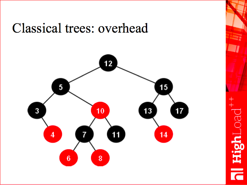
Hashes are great, but limited: data stored in a hash is unordered, so a hash is useless for range queries. As a general-purpose index, Tarantool 1.3 and 1.4 used classical trees for RAM, and they did a pretty good job, but they also had two significant drawbacks: first, each node of a typical balanced binary tree holds two pointers, or 16 bytes per value, which is an awful overhead that we wanted to avoid; and second, unsatisfactory balance. Even AVL-trees are relatively well-balanced, but compared to B-trees, which I’ll be talking about later, the number of comparisons one had to make when searching was some 30-40% higher. Not to mention that binary tree search is awful for the CPU cache prefetch: each time you traverse a tree, you’re likely to need a cache line that your cache doesn’t have, because the nodes may be scattered all over the address space, which means you can’t definitely tell the predictor what address you’re going to need. That’s why we implemented our own B+*-trees for memory.
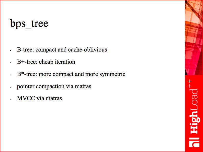
We often get asked how much faster Tarantool is than std::map in C++. In short, it is faster, but I’ll get to it later. More importantly, our system is more scalable than std::map thanks to the data structure I will now describe.
The idea behind these trees is as follows. Each tree node stores, on average, between 20 and 40 elements. We ensure that each node is well aligned in the CPU cache so that we can search within a single node without switching between cache lines.
We store elements only in leaf nodes to keep the tree header as compact as possible and make it fit in the CPU cache. To speed up tree traversal, we only iterate over the leaves without going back to the parent nodes or the root each time. And we use the matras for allocation to be able to freeze such trees and to ensure that leaf pointers take only 32, rather than 64, bits.
Here’s a somewhat awkward illustration:
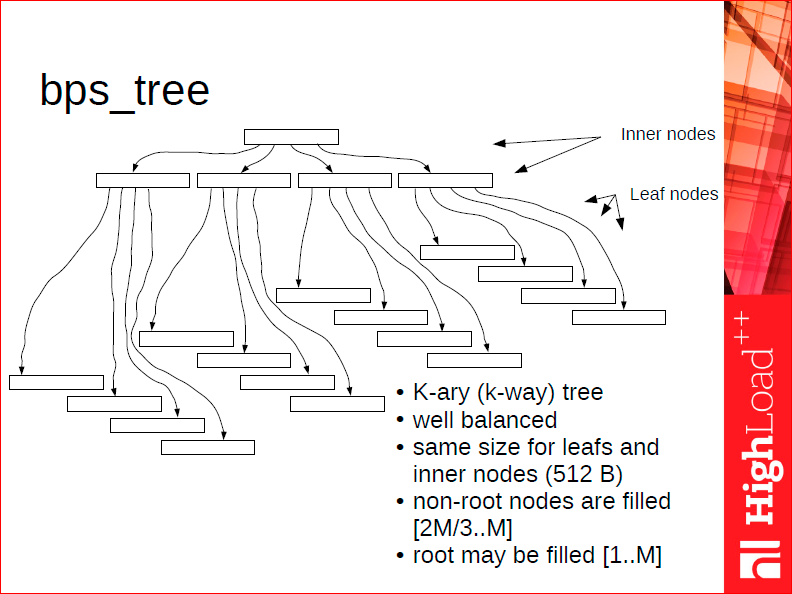
On average, given a more or less manageable size of the database, it’s a very well-balanced k-way 3-level tree.
To understand why it’s well balanced, let’s recall the difference between a B+-tree or a B+*-tree and a classical B-tree that stores data in non-terminal nodes. A B+-tree guarantees that each block is 2/3 full. That’s a classical law: if you want each block to be 1/2 full, then, when rebalancing your tree, it’s enough to somehow rearrange the elements between the current node (on average, 1/2 full) and its neighbor (on average, 1/2 full as well). If, after the rebalancing, some elements don’t fit in a node, you definitely have to split it, and you’ll still keep the 1/2 fullness. When we’re dealing with blocks that are 2/3 full, the situation with rebalancing is different: you need to take into account not one, but possibly two or even three neighboring nodes, which would depend on your configuration, and distribute the elements evenly between them. There are about 8 different cases to handle, but the resulting tree is very well balanced.
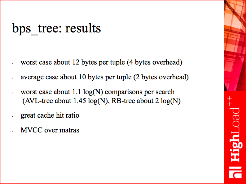
We enjoy a low overhead per storage unit and a very good balance: on average, it’s just 1.1 log(N) comparisons per search operation. Moreover, search is pretty cache-efficient since all top-level tree blocks fit in the cache.
In fact, our tree performs so well that sometimes we don’t even understand what’s faster, a hash or the B+*-tree in Tarantool 1.6. According to our measurements, a hash is still some 30-40% faster, but it’s a mere 40% gain given the logarithmic complexity of our tree against the constant complexity of a hash: this logarithm is expressed in terms of only 2 or 3 cache line lookups, whereas a hash may have an average value of 2 cache line lookups. This is another manifestation of the fact that for an in-memory database, the cost is defined not through regular operations, but rather in terms of how well a particular data structure works with the cache.
These are just a few of the data structures we implemented and use in Tarantool to achieve great performance. These structures would not be as efficient without a careful top-down design, which is only possible when creating a new database system from scratch. With this, I conclude the fourth part of my talk. I hope you enjoyed it, and if you want to know more, try playing with Tarantool - and see how well it performs in your case.